Analyzing Feature Effects

Are the relationships between features and targets sufficiently clear to diagnose and address issues effectively?
What
Understanding how individual features impact the target prediction, taking into account the nuanced and complex interactions, as well as the main effects of each feature.
How
This section introduces methods to explore practical tools for analyzing feature effects in depth, as detailed in Molnar's Interpretable Machine Learning (2023).
Individual Conditional Expectation (ICE) Plots
ICE lines represent how changes to a feature value changes a prediction. The way that an ICE line is generated is actually quite simple:
- Define a grid: Decide on a set of equally spaced values for a feature of interest, a 1-dimensional grid (let's say there are n values).
- Select a random observation: Choose an observation from your dataset at random.
- Duplicate and manipulate the observation: Make n copies of the observation, changing the feature value of each copy of the observation to one of the feature values of the grid.
- Make predictions: Predict the target value for each copy of the observation.
- Plot the ICE line: Then you just plot the feature values against the predictions as a line plot.
- Repeat for more ICE lines: Repeat this process as many times as you would like to have the number of lines you'd like. Of course, if there are too many lines, then it could become difficult to understand the plot.
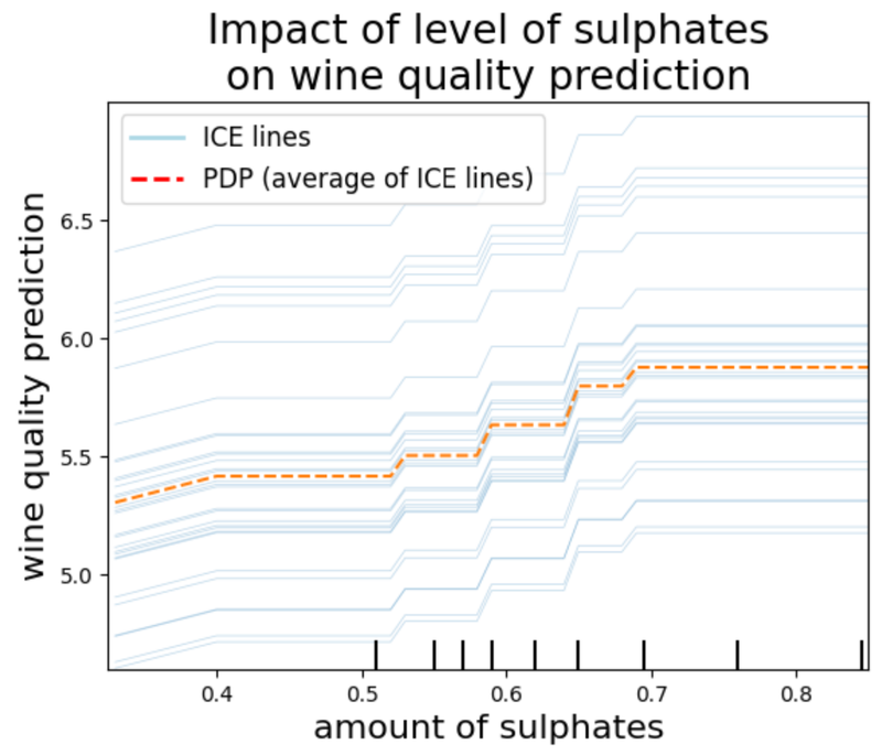
Image created by Ari Tal using an iPython Notebook, 2023
ICE lines offer granular insights into the diverse ways features affect predictions across individual data points, uncovering heterogeneous effects (i.e. the same change in the value of the feature of interest could have differing effects on the target for different observations) and feature interactions.
These plots are also instrumental in unveiling the existence of unknown feature interactions, indicated by heterogeneous effects on the target by the same value changes in the feature. This offers a nuanced perspective that can complement PDPs and ALE plots.
Advantages: Illuminate observation-level feature effects and interactions, offering detailed insights into heterogeneous effects.
Disadvantages: Can be complex to interpret due to the level of detail and potential overlap of plotted lines.
Partial Dependence Plots (PDPs)
PDPs illustrate the effect of a feature on the predicted outcome, averaging out the influences of all other features. This is done by substituting in a particular feature value into every observation of the dataset and calculating the average prediction. Repeat this process for a pre-determined number of equally spaced grid values of the feature. PDPs offer a more simplified interpretation than ICE plots by plotting just 1 line, the average of all other ICE lines.
Advantages: Easy to implement and interpret, offering clear insights into feature effects. This makes it very useful when communicating with stakeholders.
Disadvantages: Can be misleading due to the assumption of feature independence.
Accumulated Local Effects (ALE) Plots
Provide insights into feature effects, giving a more reliable representation than PDPs by indirectly compensating for feature correlations. This is how ALE is calculated for a pair of values of feature j:

These are the steps for understanding the formula:
- Determine grid values: Similar to PDPs, ALE utilizes a pre-determined equally spaced grid of values for feature j.
- Pick observations: For each each pair of consecutive grid values, you take a group of observations such that
lower grid value < feature j's value < higher grid value. - Duplicate dataset: Duplicate the group of observations. With one copy of each observation, replace the value of feature j with the higher grid value. With the other copy of the observation, replace the value of feature j with the lower grid value.

Image created by Ari Tal using an iPython Notebook, 2023
- Make predictions: For each observation, calculate the prediction for the copy of the observation with the higher grid value, prediction(observation with higher grid value), and the prediction for the copy of the observation with the lower grid value, prediction(observation with lower grid value).
- Calculate ALE value: ALE(lower grid value, higher grid value) = mean of all such differences.
- Repeat: Repeat this process for all such consecutive pairs of grid values.
- Plot ALE values: Plot each of the ALE values to see how increasing the ALE value from the lower grid value to the higher grid value changes the prediction.
Advantages: Offers a more accurate representation of feature effects due to the use of more realistic synthetic data for the calculations. This is especially important in decreasing bias when there are correlated features.
Disadvantages: Interpretation can be complex, especially in the context of strongly correlated features (even though ALE is the preferred tool when the feature(s) of interest is (are) correlated with another feature).
Friedman’s H-Statistic
Though each of the above techniques can be used to better understand specific interactions, the H-Statistic was designed for it. It quantifies the interaction strength between features, providing a statistical measure of feature interactions, which can be critical in models where interactions are suspected or known to be important.
Though I won't go through the details of the calculation, it utilizes taking the partial dependence of two features at once (thus combining the marginal effect of 1 feature, the marginal effect of the other feature, and the interaction effect) and then subtracting the partial dependence of each of the individual features, thus leaving just the interaction effect.
Advantages: Provides a quantitative measure of feature interactions.
Disadvantages: Interpretation can be non-intuitive and requires a statistical understanding to contextualize results properly.
When
Feature effect analysis becomes pivotal under specific conditions:
- When the model's performance is unsatisfactory or inconsistent.
- In the presence of unexpected predictions, indicating potential issues or hidden insights.
- When dealing with high-stakes predictions, where feature influence requires close scrutiny.
- In scenarios demanding transparency and comprehensive insights for stakeholder communication.
When these tools might not be needed:
- For features with low importance or minimal impact on predictions.
- When the model consistently performs well and meets expectations.
Potential Impacts
These techniques can highlight unintended biases, inspire confidence in the model’s adaptability to new scenarios, and guide strategic adjustments to meet broader goals and ethical norms. These tools are not always mandatory but can be indispensable for:
- Pre-Processing Enhancements: Learn about problems with your data by identifying problems with your model.
- Data Collection Guidance: Pinpoint areas lacking data coverage, directing targeted data gathering (or maybe changes to the weight of certain observations during training) to enhance representation and thus model performance.
- Model Refinement: Identifying problems with your model can inform adjustments in feature engineering, algorithm selection, and hyperparameter selection to exploit data relationships more effectively.
- Aid in Debugging: Such as diagnosing causes of unexpected behavior (Molnar, 2023).
- Boost in Stakeholder Engagement: Enhance transparency and enable informed discussions with stakeholders.
- Model Vulnerability Identification: Illuminate a model’s vulnerable spots, contributing to informed risk management strategies.
- Feature Interaction Insights: Utilize ICE plots and the H-Statistic to reveal both simple and complex interactions between features (Molnar, 2023). These tools could potentially identify unexpected relationships influencing predictions and allow for a more complete understanding of model behavior.
Transition to Next Section
Having delved into the intricacies of feature effects and how they each influence model predictions, our focus now becomes even more granular by inspecting individual predictions. The following section will introduce tools to parse a single outcome, validating that each decision is rational, transparent, fair, and actionable. This close-up view is paramount when decisions carry significant weight.